Dasymetric interpolation using CNEFE addresses
Source:vignettes/articles/tracts_to.Rmd
tracts_to.RmdCensus data in Brazil are published at the census tract level. However, many research and planning applications require data at different spatial granularities, such as hexagonal grids for standardized spatial analysis, or custom polygons such as traffic zones for transportation modeling.
tracts_to_h3() and tracts_to_polygon()
perform dasymetric interpolation using CNEFE dwelling
points as ancillary data. Instead of assuming uniform distribution
within tracts, they allocate tract-level values to individual dwelling
points identified in the CNEFE and then aggregate these to the target
spatial units. The allocation rule depends on the variable type:
-
Sum variables (e.g.,
pop_ph,race_preta,age_70m): the tract total is divided equally among eligible dwelling points. The target spatial unit (e.g., hexagons, traffic zones, or any user-supplied polygon) receives the sum of all point-level shares that fall within it. -
Average variables (
avg_inc_resp): the tract-level average is assigned (not split) to each eligible dwelling point. The target spatial unit receives the average of all assigned values within it.
This approach preserves the heterogeneous distribution of dwellings within each tract, yielding more accurate estimates than simple areal interpolation.
This article demonstrates both functions: tracts_to_h3()
for transferring census variables to an H3 hexagonal grid in Fortaleza,
and tracts_to_polygon() for transferring census variables
to traffic zones in São Paulo.
The currently supported variables (and their respective IBGE census
tract codes) can be found using the tracts_variables_ref
dataframe that accompanies the package:
library(cnefetools)
tracts_variables_ref |>
knitr::kable()| var_cnefetools | code_var_ibge | desc_var_ibge | table_ibge |
|---|---|---|---|
| pop_ph | V00005 | Domicilios Particulares Permanentes Ocupados, Quantidade de moradores | Domicilios |
| pop_ch | V00007 | Domicilios Coletivos Com Morador, Quantidade de moradores | Domicilios |
| male | V01007 | Sexo masculino | Pessoas |
| female | V01008 | Sexo feminino | Pessoas |
| age_0_4 | V01031 | 0 a 4 anos | Pessoas |
| age_5_9 | V01032 | 5 a 9 anos | Pessoas |
| age_10_14 | V01033 | 10 a 14 anos | Pessoas |
| age_15_19 | V01034 | 15 a 19 anos | Pessoas |
| age_20_24 | V01035 | 20 a 24 anos | Pessoas |
| age_25_29 | V01036 | 25 a 29 anos | Pessoas |
| age_30_39 | V01037 | 30 a 39 anos | Pessoas |
| age_40_49 | V01038 | 40 a 49 anos | Pessoas |
| age_50_59 | V01039 | 50 a 59 anos | Pessoas |
| age_60_69 | V01040 | 60 a 69 anos | Pessoas |
| age_70m | V01041 | 70 anos ou mais | Pessoas |
| race_branca | V01317 | Cor ou raca e branca | Pessoas |
| race_preta | V01318 | Cor ou raca e preta | Pessoas |
| race_parda | V01320 | Cor ou raca e parda | Pessoas |
| race_amarela | V01319 | Cor ou raca e amarela | Pessoas |
| race_indigena | V01321 | Cor ou raca e indigena | Pessoas |
| n_resp | V06001 | Pessoas responsaveis em domicilios particulares permanentes ocupados | ResponsavelRenda |
| avg_inc_resp | V06004 | Valor do rendimento nominal medio mensal das pessoas responsaveis com rendimentos por domicilios particulares permanentes ocupados | ResponsavelRenda |
Part 1: Census variables on H3 hexagons (Fortaleza)
We interpolate three census variables to H3 resolution 8 hexagons for Fortaleza (IBGE code 2304400):
-
pop_ph: population in private households -
avg_inc_resp: average income of household heads -
race_preta: population self-identified as Black (preta)
ftl_h3 <- tracts_to_h3(
code_muni = 2304400,
h3_resolution = 8,
vars = c("pop_ph", "avg_inc_resp", "race_preta")
)
#> ℹ Processing code 2304400
#>
ℹ Step 1/6: connecting to DuckDB and loading extensions...
✔ Spatial extension loaded
#> ℹ Step 1/6: connecting to DuckDB and loading extensions...
✔ Step 1/6 (DuckDB ready) [525ms]
#>
ℹ Step 2/6: preparing census tracts in DuckDB...
ℹ Using cached file: 'sc_23.parquet'
#> ℹ Step 2/6: preparing census tracts in DuckDB...
✔ Step 2/6 (Tracts ready) [372ms]
#>
ℹ Step 3/6: preparing CNEFE points in DuckDB...
ℹ Using cached file: C:\Users\jorge\AppData\Local/R/cache/R/cnefetools/2304400_FORTALEZA.zip
#> ℹ Step 3/6: preparing CNEFE points in DuckDB...
✔ Step 3/6 (CNEFE points ready) [4s]
#>
ℹ Step 4/6: spatial join (points to tracts) and allocation prep...
✔ Step 4/6 (Join and allocation) [1.2s]
#>
ℹ Step 5/6: aggregating allocated values to H3 cells...
✔ Step 5/6 (Hex aggregation) [251ms]
#>
ℹ Step 6/6: building H3 grid and joining results...
✔ Step 6/6 (sf output) [3.3s]
#>
#> ── Dasymetric interpolation diagnostics ──
#>
#> ── Stage 1: Tracts → CNEFE points
#> ! Unallocated total for population from private households (pop_ph): 2169 of
#> 2424722 (0.09%)
#> ! Unallocated total for race_preta (race_preta): 74 of 170887 (0.04%)
#> ! avg_inc_resp assigned to 1032500 of 1033952 eligible points (99.86% of total
#> points)
#> ! avg_inc_resp is NA in 128 of 4408 tracts (2.90% of total tracts)
#> ! Unmatched CNEFE points (no tract): 194 of 1034611 points (0.02% of total
#> points)
#> ! Tracts with NA totals: pop_ph in 128 of 4408 tracts (2.90% of total tracts);
#> race_preta in 200 of 4408 tracts (4.54% of total tracts)
#> ! Tracts with no eligible dwellings: pop_ph in 6 of 4408 tracts (0.14% of total
#> tracts); race_preta in 6 of 4408 tracts (0.14% of total tracts)
#>
#> ── Stage 2: CNEFE points → H3 hexagons
#> ℹ CNEFE points mapped to H3 cells: 1034417 of 1034417 allocated points
#> (100.00%)
head(ftl_h3)
#> Simple feature collection with 6 features and 4 fields
#> Geometry type: POLYGON
#> Dimension: XY
#> Bounding box: xmin: -38.54958 ymin: -3.899435 xmax: -38.48939 ymax: -3.854262
#> Geodetic CRS: WGS 84
#> id_hex pop_ph avg_inc_resp race_preta
#> 1 8880104017fffff 519.04462 2126.606 43.431126
#> 2 8880104031fffff 0.00000 NA 0.000000
#> 3 8880104033fffff 1241.65429 1623.636 122.037929
#> 4 8880104037fffff 149.32009 1329.010 8.075055
#> 5 888010403bfffff 58.81569 1281.817 7.224510
#> 6 8880104083fffff 0.00000 NA 0.000000
#> geometry
#> 1 POLYGON ((-38.51443 -3.8994...
#> 2 POLYGON ((-38.49651 -3.8962...
#> 3 POLYGON ((-38.50237 -3.8893...
#> 4 POLYGON ((-38.49341 -3.8877...
#> 5 POLYGON ((-38.50547 -3.8978...
#> 6 POLYGON ((-38.54373 -3.8646...Mapping the results
We use leafsync::sync() to display the three variables
side by side:
map_pop <- mapview(
ftl_h3,
zcol = "pop_ph",
layer.name = "Population"
)
map_inc <- mapview(
ftl_h3,
zcol = "avg_inc_resp",
layer.name = "Avg. income"
)
map_race <- mapview(
ftl_h3,
zcol = "race_preta",
layer.name = "Black pop."
)
sync(map_pop, map_inc, map_race, ncol = 3)Exploring the relationship between income and racial composition
We can examine the relationship between average household head income and the proportion of Black population in each hexagon:
ftl_h3_plot <- ftl_h3 |>
st_drop_geometry() |>
filter(pop_ph > 0) |>
mutate(pct_preta = race_preta / pop_ph)
ggplot(ftl_h3_plot, aes(x = avg_inc_resp, y = pct_preta)) +
geom_point(alpha = 0.3, size = 3) +
geom_smooth(method = "loess", se = TRUE, color = "steelblue") +
scale_y_continuous(labels = scales::percent_format()) +
labs(
x = "Average income of household heads (R$)",
y = "Black population share (race_preta / pop_ph)"
) +
theme_minimal()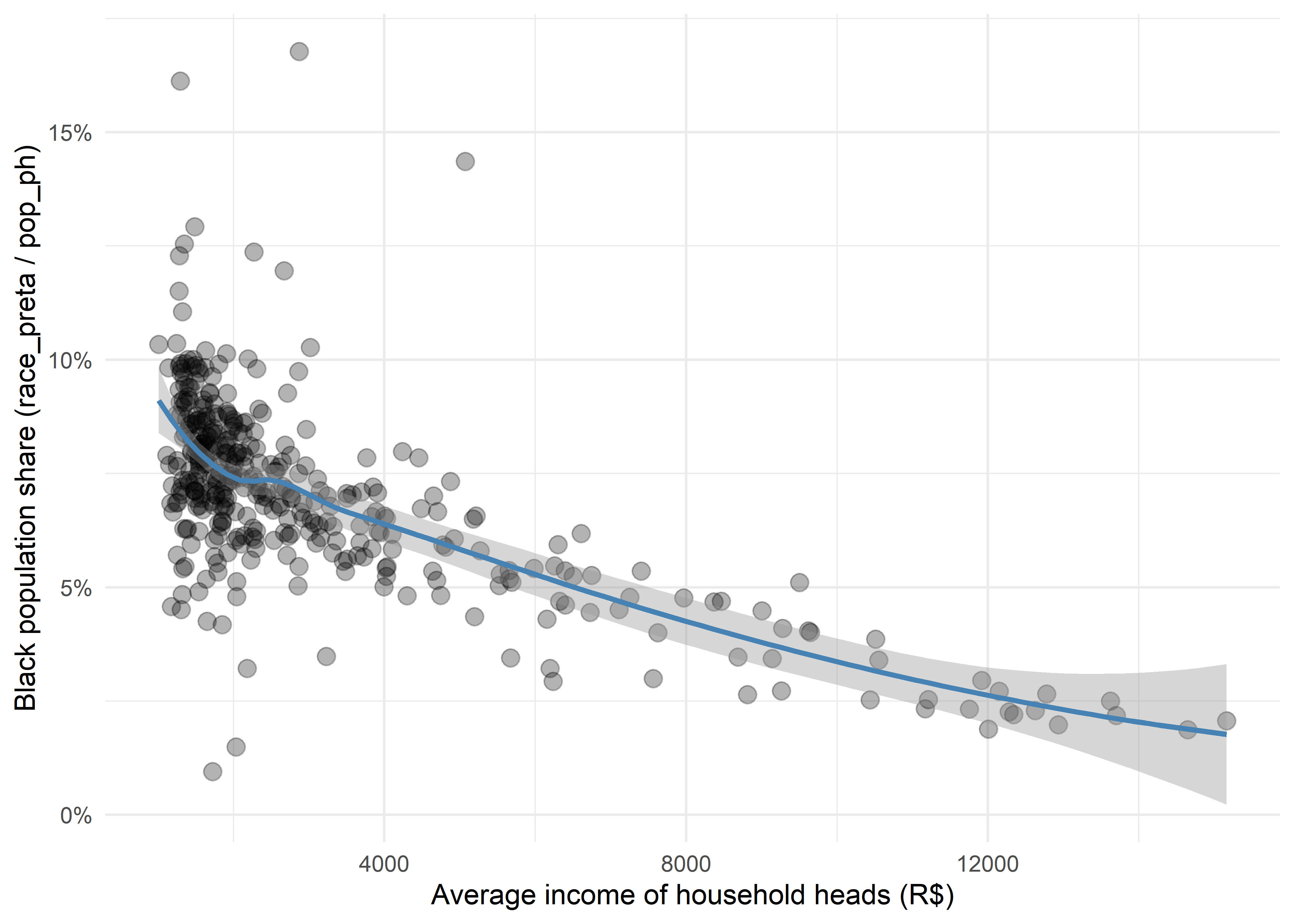
As expected, the plot reveals a strong negative correlation between these two variables: hexagons with lower average household income tend to have a substantially higher share of Black population. This pattern reflects deep-rooted racial income inequality, a persistent feature of the Brazilian social landscape.
Part 2: Census variables on traffic zones (São Paulo)
Transportation planning often requires census-derived variables at
the traffic zone level rather than the census tract level. The odbr package
provides traffic zone geometries from origin-destination surveys
conducted in Brazilian metropolitan areas. Since the OD survey for São
Paulo covers the entire metropolitan region (39 municipalities), we
filter only the traffic zones within the municipality of São Paulo.
library(odbr)
# Load traffic zones for the São Paulo metropolitan region
sp_zones <- read_map(
city = "Sao Paulo",
year = 2017,
geometry = "zone"
)
# Filter zones within the municipality of São Paulo
sp_zones_muni <- sp_zones |>
filter(NomeMunici == "São Paulo") |>
sf::st_make_valid() # Correcting invalid geometries in advance
nrow(sp_zones_muni)
#> [1] 342We interpolate two variables:
-
pop_ph: population in private households -
age_70m: population aged 70 years or older
sp_zones_census <- tracts_to_polygon(
code_muni = 3550308,
polygon = sp_zones_muni,
vars = c("pop_ph", "age_70m")
)
#> ℹ Processing municipality code 3550308...
#>
ℹ Step 1/6: aligning CRS...
ℹ Input CRS: "EPSG:22523" | Output CRS: "EPSG:22523"
#> ℹ Step 1/6: aligning CRS...
✔ Step 1/6 (CRS alignment) [359ms]
#>
ℹ Step 2/6: connecting to DuckDB and loading extensions...
✔ Spatial extension loaded
#> ℹ Step 2/6: connecting to DuckDB and loading extensions...
✔ Step 2/6 (DuckDB ready) [567ms]
#>
ℹ Step 3/6: preparing census tracts in DuckDB...
ℹ Using cached file: 'sc_35.parquet'
#> ℹ Step 3/6: preparing census tracts in DuckDB...
✔ Step 3/6 (Tracts ready) [5.1s]
#>
ℹ Step 4/6: preparing CNEFE points in DuckDB...
ℹ Using cached file: C:\Users\jorge\AppData\Local/R/cache/R/cnefetools/3550308_SAO_PAULO.zip
#> ℹ Step 4/6: preparing CNEFE points in DuckDB...
✔ Step 4/6 (CNEFE points ready) [18.1s]
#>
ℹ Step 5/6: spatial join (points to tracts) and allocation...
✔ Step 5/6 (Join and allocation) [15.1s]
#>
ℹ Step 6/6: aggregating allocated values to polygons...
✔ Step 6/6 (Polygon aggregation) [377ms]
#>
#> ── Dasymetric interpolation diagnostics ──
#>
#> ── Stage 1: Tracts → CNEFE points
#> ! Unallocated total for population from private households (pop_ph): 86998 of
#> 11394071 (0.76%)
#> ! Unallocated total for age_70m (age_70m): 5397 of 923921 (0.58%)
#> ! Unmatched CNEFE points (no tract): 2935 of 4996529 points (0.06% of total
#> points)
#> ! Tracts with NA totals: pop_ph in 622 of 27301 tracts (2.28% of total tracts);
#> age_70m in 1316 of 27301 tracts (4.82% of total tracts).
#> ! Tracts with no eligible dwellings: pop_ph in 324 of 27301 tracts (1.19% of
#> total tracts); age_70m in 297 of 27301 tracts (1.09% of total tracts)
#>
#> ── Stage 2: CNEFE points → Polygons
#> ℹ Polygon coverage: 4993321 of 4993594 allocated points captured (99.99%)
#> ℹ Polygons with no CNEFE points: 3 of 342 total polygons (0.88%)
head(sp_zones_census)
#> Simple feature collection with 6 features and 9 fields
#> Geometry type: POLYGON
#> Dimension: XY
#> Bounding box: xmin: 331820.5 ymin: 7393922 xmax: 334180.5 ymax: 7396311
#> Projected CRS: Corrego Alegre 1970-72 / UTM zone 23S
#> # A tibble: 6 × 10
#> NumeroZona NomeZona NumeroMuni NomeMunici NumDistrit NomeDistri Area_ha_2
#> <dbl> <chr> <dbl> <chr> <dbl> <chr> <dbl>
#> 1 1 Sé 36 São Paulo 80 Sé 57.1
#> 2 2 Parque Dom P… 36 São Paulo 80 Sé 114.
#> 3 3 Praça João M… 36 São Paulo 80 Sé 47.8
#> 4 4 Ladeira da M… 36 São Paulo 67 República 75.1
#> 5 5 República 36 São Paulo 67 República 75.0
#> 6 6 Santa Ifigên… 36 São Paulo 67 República 82.9
#> # ℹ 3 more variables: geom <POLYGON [m]>, pop_ph <dbl>, age_70m <dbl>Mapping the elderly population share
We compute the share of population aged 70+ in each traffic zone. This indicator is relevant for identifying areas where transport planning should prioritize accessibility for people with reduced mobility, such as low-floor buses, accessible sidewalks, and demand-responsive transit services.
Notes
Notice how tracts_to_polygon() is particularly useful in
transportation research, where census variables (such as population by
age group and income) are essential inputs for travel demand models
(especially in Trip Generation models from 4-Step modeling). However,
traffic zone geometries rarely align with census tract boundaries.
Dasymetric interpolation via CNEFE dwelling points provides a principled
method to bridge this spatial mismatch, transferring census data to
custom spatial units and supporting more accurate trip generation and
distribution models.
Hint to scaling to multiple municipalities
The odbr traffic zones cover the entire São Paulo
metropolitan region (39 municipalities). To interpolate census data for
all municipalities, you can use purrr::map() to apply
tracts_to_polygon() to each municipality and then combine
the results with dplyr::bind_rows().
Future versions
In future versions of the package, tracts_to_polygon()
will support municipality-independent operation, allowing users to pass
polygons that span multiple municipalities without the need for
per-municipality iteration.
Interpolation diagnostics
Both functions print detailed diagnostics after each run, so the user
can assess the quality of the interpolation. For example, the
tracts_to_h3() call for Fortaleza above produces:
── Dasymetric interpolation diagnostics ──
! Unallocated total for population from private households (pop_ph): "2169" ("0.09%" of total)
! Unallocated total for race_preta (race_preta): "74" ("0.04%" of total)
! avg_inc_resp assigned to 1032500 of 1033953 eligible points
! avg_inc_resp is "NA" in 128 tracts
! Unmatched CNEFE points (no tract): 194
! Tracts with "NA" totals: pop_ph "NA" in 128; race_preta "NA" in 200
! Tracts with no eligible dwellings: pop_ph in 6 tracts; race_preta in 6 tractsAnd the tracts_to_polygon() call for São Paulo:
── Dasymetric interpolation diagnostics ──
! Unallocated total for population from private households (pop_ph): "86998" ("0.76%" of total)
! Unallocated total for age_70m (age_70m): "5397" ("0.58%" of total)
! Unmatched CNEFE points (no tract) = 2935
! Tracts with "NA" totals: pop_ph "NA" in 622; age_70m "NA" in 1316
! Tracts with no eligible dwellings: pop_ph in 324 tracts; age_70m in 297 tractsThese warnings report the amount of unallocated population (and its percentage of the census total), the number of CNEFE points that could not be matched to a tract, and the number of tracts with missing values or no eligible dwellings. In both examples, the unallocated shares are small (below 1%), indicating that the interpolation preserves most of the original census totals. Users should inspect these diagnostics to decide whether the loss is acceptable for their application.
Ecological fallacy caveat
Dasymetric interpolation distributes tract-level aggregates to dwelling points under the assumption that each dwelling within a tract receives an equal share of the total. This means that the method does not recover true individual- or dwelling-level values; it redistributes a group statistic. Drawing conclusions about individuals from such aggregated data constitutes an ecological fallacy (the error of attributing group-level patterns to individuals).
The risk is greater when the source census tracts are large, since larger tracts are more likely to contain internally heterogeneous populations, making the uniform allocation assumption less realistic. Users should interpret interpolated values as spatial estimates of aggregate quantities, not as precise measurements at the dwelling or individual level.