Performance benchmark: DuckDB vs pure-R backends • cnefetools

Introduction

Under the hood, {cnefetools} uses DuckDB as its default backend to perform spatial operations efficiently, with speedups of up to 20x over pure-R code depending on the number of address points and the size of the spatial units.

This performance boost is made possible by three DuckDB extensions:

spatial: performs spatial joins (e.g., point-in-polygon) in SQL
zipfs: reads CSV files directly from cached ZIP archives, avoiding the need to extract files to disk
h3: assigns geographic coordinates to H3 hexagonal grid cells entirely inside DuckDB

A pure-R fallback (backend = "r") is also available, using h3jsr and sf for the same operations (slower, but without the DuckDB dependency).

In this article, we demonstrate the performance in two different settings using the cnefe_counts() function:

First, we compare three different municipalities: São Paulo-SP (~5.7 million addresses), Curitiba-PR (~900,000 addresses), and Vitória da Conquista-BA (~200,000 addresses);
Then, we contrast processing times for three different H3 resolutions (7, 9, and 11) within the same city (Curitiba).

Benchmarks were run on a machine equipped with a 14-core, 20-thread CPU (13th Gen Intel Core i9-13900H, 2.60 GHz), 32 GB of RAM, and Windows 11. Tests were executed in R 4.3.2 using DuckDB 1.4.1.

Comparing cities of different sizes

Let’s compare the performance of cnefe_counts() when aggregating CNEFE address points to H3 hexagons at resolution 8.

Setup

library(cnefetools)
library(dplyr)
library(ggplot2)
library(kableExtra)

# Municipality codes
cod_spo <- 3550308 # São Paulo
cod_ctb <- 4106902 # Curitiba
cod_vca <- 2933307 # Vitória da Conquista

cods <- c(cod_spo, cod_ctb, cod_vca)

# Benchmark DuckDB backend
time_duckdb_cities <- sapply(
  cods,
  function(i){
    system.time({
      result_duckdb_cities <- cnefe_counts(
        code_muni = i,
        polygon_type = "hex",
        h3_resolution = 8,
        backend = "duckdb",
        verbose = FALSE
      )
    })
  }
)

# Benchmark pure-R backend
time_r_cities <- sapply(
  cods,
  function(i){
    system.time({
      result_duckdb_cities <- cnefe_counts(
        code_muni = i,
        polygon_type = "hex",
        h3_resolution = 8,
        backend = "r",
        verbose = FALSE
      )
    })
  }
)

# Results
benchmark_results_cities <- data.frame(
  city = rep(c("São Paulo", "Curitiba", "Vitória da Conquista"),2),
  backend = rep(c("Pure R","DuckDB"), each = 3),
  time_seconds = c(time_r_cities["elapsed",], time_duckdb_cities["elapsed",])
)

Visualization

ggplot(benchmark_results_cities
       |> mutate(
         city = factor(city, levels = c('Vitória da Conquista','Curitiba','São Paulo')),
         backend = factor(backend, levels = c("Pure R", "DuckDB")),
       ),
       aes(x = city, y = time_seconds, fill = backend)) +
  geom_col(width = 0.6, position = position_dodge(width = 0.6)) +
  geom_text(
    aes(label = sprintf("%.2f s", time_seconds)),
    position = position_dodge(width = 0.6),
    vjust = -0.4,
    size = 3
  ) +
  scale_fill_manual(values = c("Pure R" = "#E74C3C", "DuckDB" = "#2C3E50")) +
  scale_y_continuous(expand = expansion(mult = c(0, 0.08))) +
  labs(
    title = "Performance comparison: DuckDB vs Pure R",
    subtitle = "(per city)",
    y = "Execution time (seconds)",
    fill = "Backend",
    x = NULL
  ) +
  theme_minimal(base_size = 13) +
  theme(
    plot.title = element_text(face = "bold", size = 15, hjust = 0.5),
    plot.subtitle = element_text(hjust = 0.5),
    panel.grid.major.y = element_blank()
  )

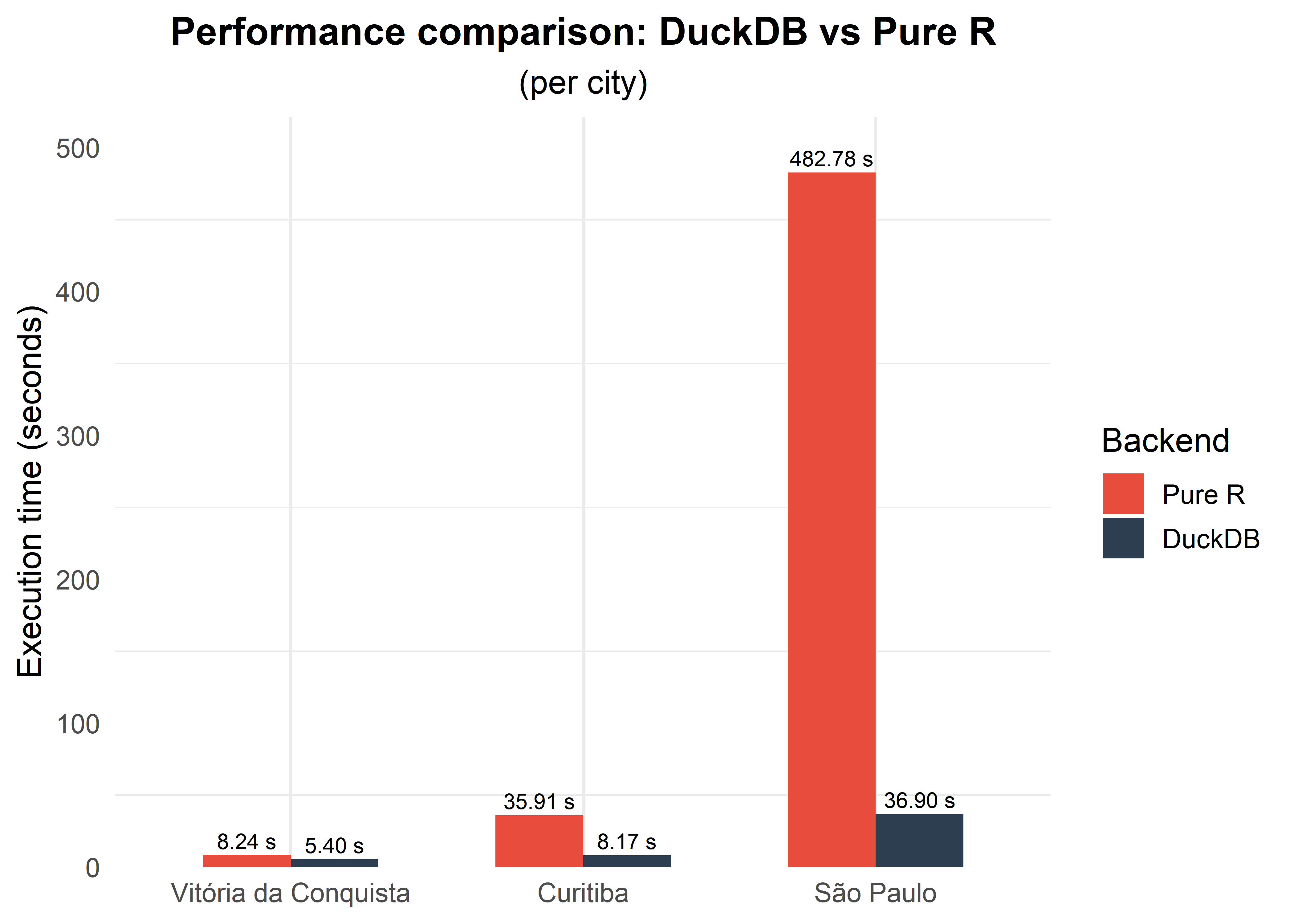
Note: For smaller municipalities, the DuckDB backend may offer little or no speedup over pure R, and in some cases may even be slightly slower. This occurs because DuckDB incurs a fixed overhead to initialize the database connection, load extensions, and materialize the data into its in-memory storage before any computation begins. When the dataset is small, this setup cost can outweigh the gains from DuckDB’s optimized query execution, making the pure-R backend competitive or faster.

Contrasting aggregation across three different spatial resolutions

Now let’s compare the performance of cnefe_counts() when aggregating CNEFE address points at different H3 resolutions for the same city.

h3_res <- c(7,9,11)

# Benchmark DuckDB backend
time_duckdb_h3 <- sapply(
  h3_res,
  function(i){
    system.time({
      result_duckdb_h3 <- cnefe_counts(
        code_muni = cod_ctb,
        polygon_type = "hex",
        h3_resolution = i,
        backend = "duckdb",
        verbose = FALSE
      )
    })
  }
)

# Benchmark pure-R backend
time_r_h3 <- sapply(
  h3_res,
  function(i){
    system.time({
      result_duckdb_h3 <- cnefe_counts(
        code_muni = cod_ctb,
        polygon_type = "hex",
        h3_resolution = i,
        backend = "r",
        verbose = FALSE
      )
    })
  }
)

# Results
benchmark_results_h3 <- data.frame(
  h3_res = rep(c(7,9,11),2),
  backend = rep(c("Pure R","DuckDB"), each = 3),
  time_seconds = c(time_r_h3["elapsed",], time_duckdb_h3["elapsed",])
)

Visualization

ggplot(benchmark_results_h3
       |> mutate(
         h3_res = as.factor(h3_res),
         backend = factor(backend, levels = c("Pure R", "DuckDB"))
         ),
       aes(x = h3_res, y = time_seconds, fill = backend)) +
  geom_col(width = 0.6, position = position_dodge(width = 0.6)) +
  geom_text(
    aes(label = sprintf("%.2f s", time_seconds)),
    position = position_dodge(width = 0.6),
    vjust = -0.6,
    size = 3
  ) +
  scale_fill_manual(values = c("Pure R" = "#E74C3C", "DuckDB" = "#2C3E50")) +
  scale_y_continuous(expand = expansion(mult = c(0, 0.08))) +
  labs(
    title = "Performance comparison: DuckDB vs Pure R",
    subtitle = "(different spatial resolutions)",
    y = "Execution time (seconds)",
    fill = "Backend",
    x = "H3 resolution"
  ) +
  theme_minimal(base_size = 13) +
  theme(
    plot.title = element_text(face = "bold", size = 15, hjust = 0.5),
    plot.subtitle = element_text(hjust = 0.5),
    panel.grid.major.y = element_blank(),
    )

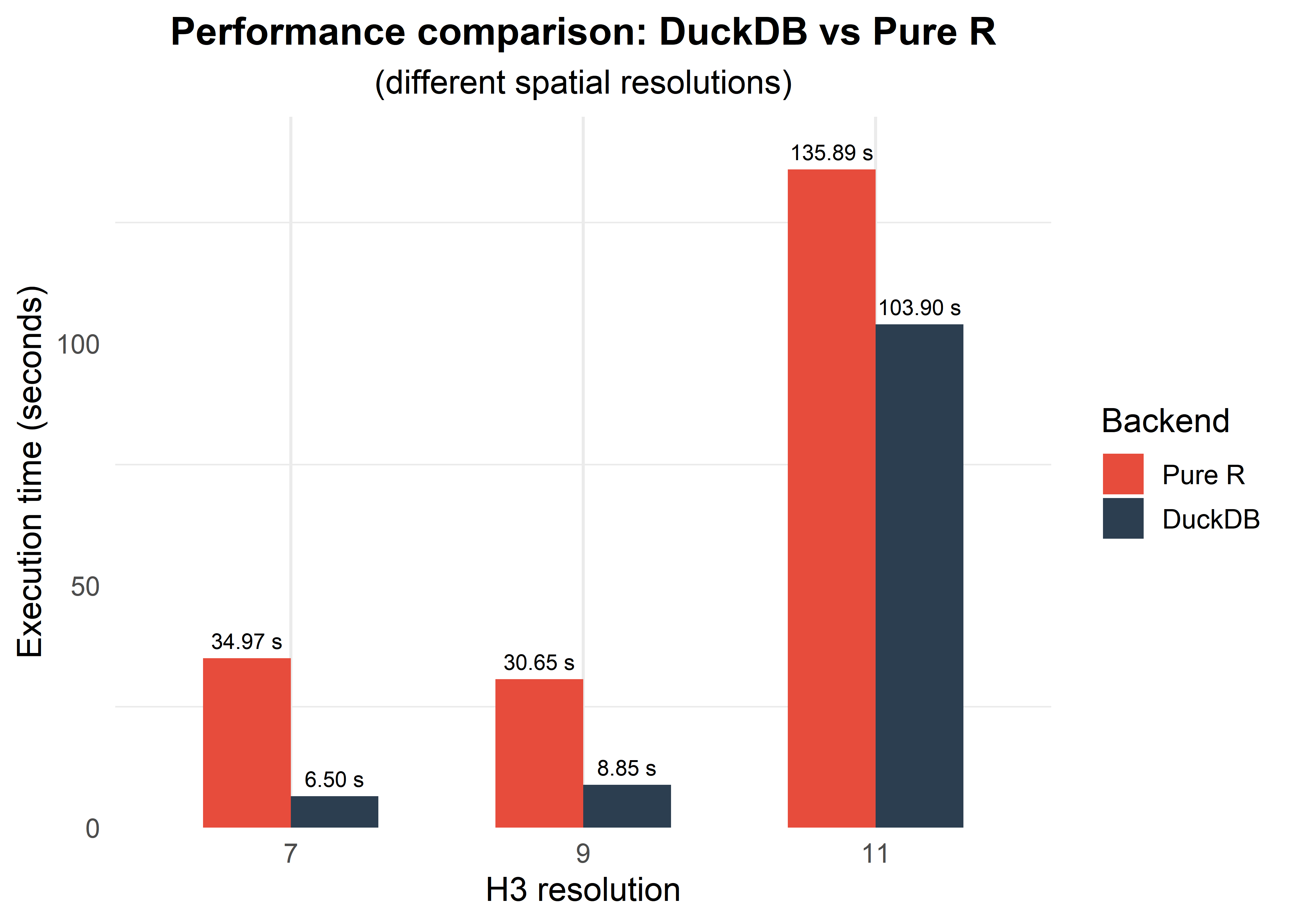
Note: At finer H3 resolutions the hexagons are much smaller, so the H3 point-to-cell indexing — which both backends ultimately delegate to the same underlying H3 C library — dominates the total runtime. Because DuckDB still pays a fixed overhead to initialize the connection, load extensions, and materialize data into its in-memory store, the relative advantage shrinks as the actual computation becomes lighter per cell. At resolution 11 this overhead can even offset DuckDB’s gains, making the pure-R backend competitive or faster.

Conclusions

The DuckDB backend is consistently faster than the pure-R implementation, and the processing time depends on:

City size (number of CNEFE addresses):

# Computing speedup for each city
speedups_cities <- benchmark_results_cities |>
  group_by(city) |>
  summarize(
    speedup = time_seconds[backend == 'Pure R']/time_seconds[backend == 'DuckDB']
    )

# Formatting output table
speedups_cities |>
  mutate(
    city = factor(city, levels = c("Vitória da Conquista", "Curitiba", "São Paulo")),
    n_points = c("~900,000", "~5,700,000", "~200,000")[match(city, c("Curitiba", "São Paulo", "Vitória da Conquista"))],
    speedup = round(speedup, 2)
  ) |>
  arrange(city) |>
  select(city, n_points, speedup) |>
  ## Improved table output with kableExtra package:
  kbl() |>
  kable_styling()

city	n_points	speedup
Vitória da Conquista	~200,000	1.53
Curitiba	~900,000	4.40
São Paulo	~5,700,000	13.08

Resolution of spatial units where CNEFE addresses are counted:

# Computing speedup for each H3 resolution
speedups_h3 <- benchmark_results_h3 |>
  group_by(h3_res) |>
  summarize(
    speedup = time_seconds[backend == 'Pure R']/time_seconds[backend == 'DuckDB']
    )

# Formatting output table
speedups_h3 |>
  mutate(
    avg_hex_area_m2 = c(5161293.36, 105332.51, 2149.64)[match(h3_res, c(7, 9, 11))],
    speedup = round(speedup, 2)
  ) |>
  select(h3_res, avg_hex_area_m2, speedup) |>
  ## Improved table output with kableExtra package:
  kbl() |>
  kable_styling()

h3_res	avg_hex_area_m2	speedup
7	5161293.36	5.38
9	105332.51	3.46
11	2149.64	1.31

Recommendation: Use the DuckDB backend (default) for best performance. The pure R backend (backend = "r") is available only if you cannot install DuckDB in your environment.