Computing land-use mix indices with CNEFE data
Source:vignettes/articles/compute_lumi.Rmd
compute_lumi.RmdLand use mix (LUM) indices quantify how different types of activities
are distributed within a spatial unit. They are widely used in urban
planning to monitor mixed-use targets, inform zoning revisions, and
prioritize transit-oriented development interventions.
compute_lumi() computes a suite of LUM indices from CNEFE
data considering a binary comparison of residential vs. non-residential
uses, aggregated either to H3 hexagonal cells or user-provided
polygons.
This article compares three of the indices produced by
compute_lumi(): the Entropy Index (EI),
the Balance Index (BAL), and the Bidirectional
Global-centered Balance Index (BGBI), proposed by Pedreira
Jr. et al. (2026). We use the municipality of São Paulo at H3 resolution
8 and produce a synchronized three-panel map using the
leafsync package.
A brief overview of the indices
All three indices are computed from the local residential share within each spatial unit , , where is the number of residential addresses and is the total number of addresses (excluding those under construction) for this spatial unit . The local non-residential share is , and the citywide residential share is denoted .
Entropy Index (EI)
EI ranges from 0 (complete homogeneity) to 1 (perfect 50/50 balance). It measures how mixed a unit is, but it does not indicate which use dominates when the unit is homogeneous: a fully residential cell and a fully non-residential cell both receive EI = 0.
Balance Index (BAL)
BAL also ranges from 0 to 1, but it defines balance relative to the observed citywide composition rather than a fixed 50/50 split. This means BAL = 1 when , not necessarily when . Like EI, however, BAL is non-directional: it does not indicate whether a low-balance cell is predominantly residential or non-residential.
Bidirectional Global-centered Balance Index (BGBI)
BGBI ranges from -1 to +1 and addresses two limitations of conventional indices:
- Directionality: positive values indicate a local residential share above the citywide reference (), while negative values indicate non-residential dominance (). This allows analysts to distinguish between functionally opposite patterns without consulting auxiliary data.
- Citywide reference: BGBI is centered at (BGBI = 0) rather than at . When the citywide composition is highly asymmetric (e.g., ), treating 50/50 as the universal balance target can distort interpretation. BGBI instead evaluates local composition against the empirically observed baseline.
Visualizing the index domains
Before generating these indices with real data, let’s examine how EI, BAL, and BGBI behave as a function of for a stylized city with , which is typical of Brazilian municipalities.
P <- 0.75 # citywide residential proportion
## BGBI function:
bgbi_fun <- function(p, P) {
((2 * p - 1) - (2 * P - 1)) / (1 - (2 * p - 1) * (2 * P - 1))
}
## EI function:
ei_fun <- function(p) {
q <- 1 - p
m <- cbind(p, q)
m[m == 0] <- NA # avoid log(0)
-rowSums(m * log(m), na.rm = TRUE) / log(2)
}
## BAL function:
bal_fun <- function(p, P) {
1 - abs(p - (P / (1 - P)) * (1 - p)) /
(p + (P / (1 - P)) * (1 - p))
}
## Generating p values between 0 and 1
p <- seq(0, 1, by = 0.01)
## Index dataframe
df_ind <- data.frame(p = p) |>
mutate(
EI = ei_fun(p),
BAL = bal_fun(p, P),
BGBI = bgbi_fun(p, P)
) |>
pivot_longer(
cols = c(EI, BAL, BGBI),
names_to = "Index",
values_to = "Value"
) |>
mutate(Index = factor(Index, levels = c("EI", "BAL", "BGBI")))
## Plotting
ggplot(df_ind, aes(x = p, y = Value, color = Index)) +
geom_line(linewidth = 0.8) +
geom_hline(yintercept = 0, linetype = "dashed", color = "gray50") +
geom_vline(xintercept = P, linetype = "dotted", color = "gray50") +
annotate("text", x = P + 0.02, y = -0.8, label = paste0("P = ", P),
hjust = 0, size = 3.5, color = "gray30") +
scale_x_continuous(
expression(p[i]),
breaks = seq(0, 1, by = 0.2)
) +
labs(y = "Index value", color = NULL) +
theme_minimal() +
theme(legend.position = "bottom")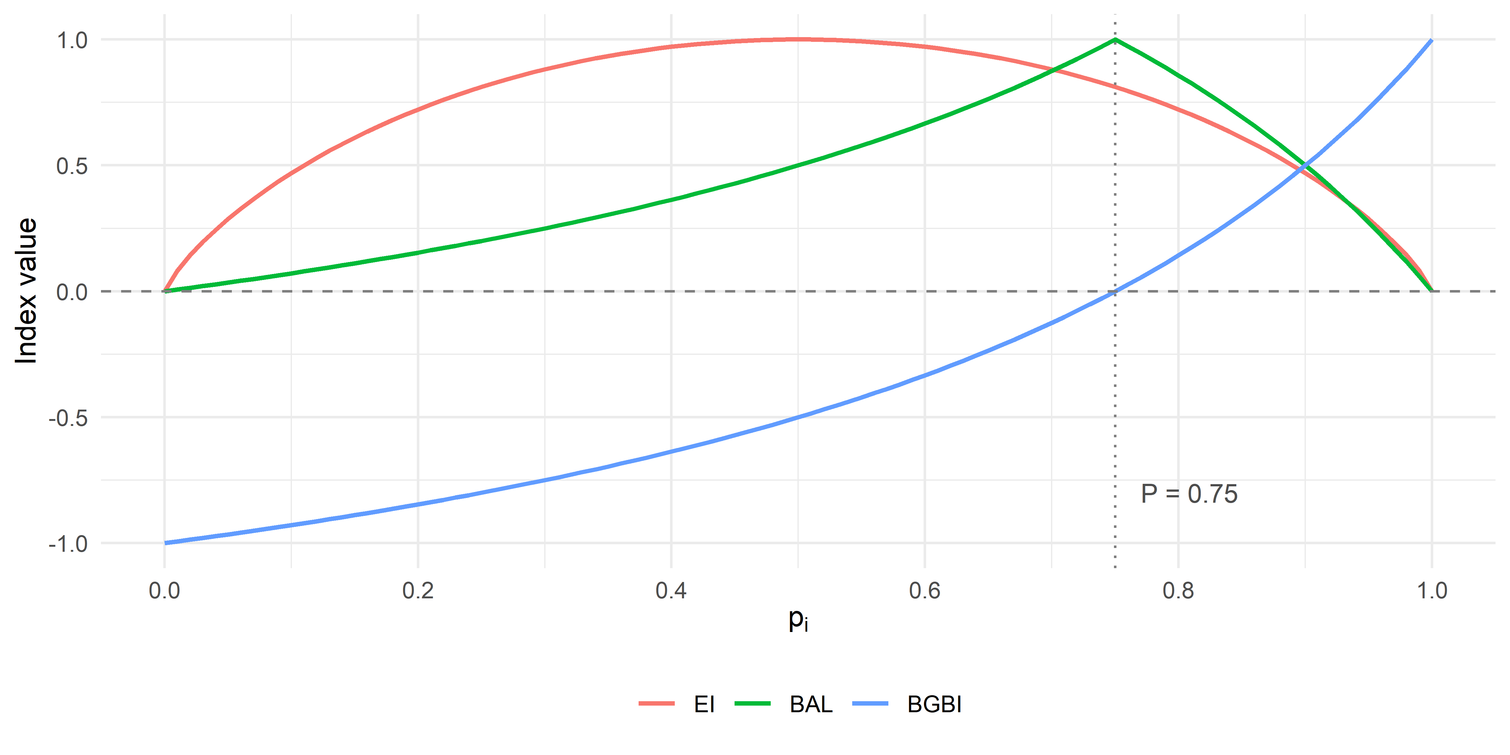
Notice that EI peaks at (the 50/50 split) and is symmetric around that point, whereas BAL peaks at (the citywide reference), reflecting its global centering. Both are non-negative and non-directional. BGBI, in contrast, crosses zero at and spans the full range, providing a signed measure that distinguishes residential-dominant from non-residential-dominant cells.
Computing the indices with compute_lumi for São Paulo
(H3 resolution 8)
spo_lumi <- compute_lumi(
code_muni = 3550308, # IBGE code for São Paulo
h3_resolution = 8
)
#> ℹ Processing municipality code 3550308...
#>
ℹ Step 1/3: Ensuring ZIP and inspecting archive...
ℹ Using cached file: C:\Users\jorge\AppData\Local/R/cache/R/cnefetools/3550308_SAO_PAULO.zip
#> ℹ Step 1/3: Ensuring ZIP and inspecting archive...
✔ Step 1/3 (CNEFE ZIP ready) [342ms]
#>
ℹ Step 2/3: Counting addresses per H3 cell...
✔ Step 2/3 (Addresses counted) [21.5s]
#>
ℹ Step 3/3: Building grid and computing LUMI...
✔ Step 3/3 (Land use mix indices computed) [2.2s]
head(spo_lumi)
#> Simple feature collection with 6 features and 8 fields
#> Geometry type: POLYGON
#> Dimension: XY
#> Bounding box: xmin: -46.64775 ymin: -23.72164 xmax: -46.61922 ymax: -23.69734
#> Geodetic CRS: WGS 84
#> id_hex p_res ei hhi bal ice hhi_adp
#> 1 88a8100001fffff 0.9277630 0.3742168 0.8659623 0.7773072 0.8555260 0.7319247
#> 2 88a8100003fffff 0.8941588 0.4872430 0.8107223 0.9829543 0.7883175 0.6214445
#> 3 88a8100005fffff 0.9271726 0.3763875 0.8649528 0.7814819 0.8543452 0.7299057
#> 4 88a8100007fffff 0.9072356 0.4456303 0.8316817 0.9099987 0.8144712 0.6633634
#> 5 88a8100009fffff 0.9493506 0.2891490 0.9038320 0.6068659 0.8987013 0.8076640
#> 6 88a810000bfffff 0.8867624 0.5096051 0.7991702 0.9791230 0.7735247 0.5983405
#> bgbi geometry
#> 1 0.22269279 POLYGON ((-46.6326 -23.7141...
#> 2 0.01704570 POLYGON ((-46.63854 -23.707...
#> 3 0.21851813 POLYGON ((-46.62338 -23.713...
#> 4 0.09000133 POLYGON ((-46.62932 -23.706...
#> 5 0.39313410 POLYGON ((-46.63588 -23.721...
#> 6 -0.02087697 POLYGON ((-46.64182 -23.715...The output includes, among others, the columns ei,
bal, and bgbi.
Mapping EI, BAL, and BGBI side by side
We use leafsync::sync() to display three maps in a
single row. EI and BAL use the default mapview palette, while BGBI uses
a diverging red-white-blue scale where red indicates non-residential
dominance (-1), white indicates citywide-referenced balance (0), and
blue indicates residential dominance (+1).
map_ei <- mapview(
spo_lumi,
zcol = "ei",
layer.name = "EI"
)
map_bal <- mapview(
spo_lumi,
zcol = "bal",
layer.name = "BAL"
)
map_bgbi <- mapview(
spo_lumi,
zcol = "bgbi",
col.regions = colorRampPalette(c("red", "white", "blue")),
layer.name = "BGBI"
)
sync(map_ei, map_bal, map_bgbi, ncol = 3)Interpreting the maps
EI and BAL highlight how mixed each hexagon is, but they cannot distinguish between hexagons dominated by residential addresses and those dominated by non-residential addresses. BGBI resolves this ambiguity by encoding the direction of deviation from the citywide baseline in its sign. This yields a three-part spatial interpretation:
- BGBI near 0 (white): the local composition is close to the citywide reference (these are balanced transition zones).
- BGBI > 0 (blue): the local residential share exceeds the citywide reference.
- BGBI < 0 (red): non-residential uses dominate relative to the citywide reference.
This directional information is especially useful when the citywide composition is highly asymmetric (as is typical in Brazilian cities, where ), because conventional indices compress most cells into a narrow range and cannot indicate the direction of homogeneity.
Producing indices for any user-supplied polygon
compute_lumi() also supports user-provided polygons via
the polygon_type = "user" argument, enabling computation of
these indices for any spatial unit of interest (such as neighborhoods,
census tracts, or health districts), depending on the specific research
or policy purpose. See the example below for the neighborhoods of
Maringá (IBGE code 4115200), downloaded with the geobr
package.
library(geobr)
mga_nei <- read_neighborhood(year = 2022) |>
filter(code_muni == 4115200) # IBGE code for Maringá
mga_lumi <- compute_lumi(
code_muni = 4115200,
polygon_type = "user",
polygon = mga_nei
)
mapview(
mga_lumi,
zcol = "bgbi",
col.regions = colorRampPalette(c("red", "white", "blue")),
layer.name = "BGBI"
)Notes on user-supplied polygons
- If
polygonis provided butpolygon_typeis not explicitly set to"user", the function automatically switches topolygon_type = "user"and issues a warning at the beginning of the processing. - The CRS of the output layer matches the CRS of the layer supplied in
polygon. If a different CRS is desired, it can be specified via thecrs_outputargument.
Notes
In addition to EI, BAL, and BGBI, compute_lumi() also
produces the Index of Concentration at the Extremes (ICE), the
Herfindahl–Hirschman Index (HHI), and an adapted HHI (aHHI), which
converts the HHI into a directional index (Pedreira Jr. et al., 2026).
All indices are returned in a single output, allowing comprehensive
comparisons within the same workflow.
References
Pedreira Jr., J. U.; Louro, T. V.; Assis, L. B. M.; Brito, P. L.; Bomfim, F. G. (2026). BGBI: A citywide-referenced and bidirectional land use mix index for planning and policy evaluation. Land Use Policy, 169, 108135. https://doi.org/10.1016/j.landusepol.2026.108135